COUNTIF function in Excel
Those that only use Excel for creating tables by hand are missing out on the many benefits of the Microsoft tool. The variety of functions makes your work easier – both at home and in the office. However, to take advantage of the Excel benefits, you need to understand the individual functions. One of the many useful tools is the COUNTIF function. Find out more about how to use the function correctly and what you might need it for.
- Up to 50 GB Exchange email account
- Outlook Web App and collaboration tools
- Expert support & setup service
What is COUNTIF used for?
Imagine you have an unsorted list of entries that might include, for example, a few months’ sales figures, and you want to find out how often a specific item has been sold. Instead of manually sorting through the list, use the COUNTIF function. The function ensures that cells with a certain value are counted.
In Excel, COUNTIF is a statistical function. As the application examples show, the function is used to create statistics. For example, by finding out how often item XY is sold, it’s easy to tell which items are the most popular. The statistical data can then be used to create visual components such as diagrams and graphs.
The COUNTIF function in Excel is basically a combination of the IF function and the COUNT function or the COUNTA function (statistical function).The combination ensures that Excel only counts a cell if certain criteria are met.
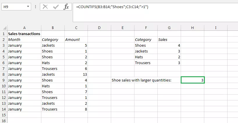
Do not confuse COUNTIF with SUMIF: the similar function does not give the number of entries of a particular value and within a certain range, but rather totals the entries within a certain range. In our example below, the corresponding item was sold in larger quantities for each sales promotion. SUMIF determines how many individual products were eventually sold.
Learn more about "Count characters in Excel" in our Digital Guide/ Startup Guide article on the topic.
How does it work? COUNTIF in use
With Excel functions, it’s very important to use the right syntax:
=COUNTIF(Range;Search criterion)
The term range signifies the cells in your table that contain the data you wish to be counted. The term search criterion signifies the corresponding value to be taken into account. The range should include a beginning and endpoint, separated by a colon. In other words, ‘B3:B14’ includes the two mentioned cells as well as all cells that come between them. Alternatively, you can create a range by dragging the mouse and highlighting the corresponding cell range. It is also possible to select an entire column: simply enter the column as the range and no lines – ‘B:B’. This technique also works for rows.
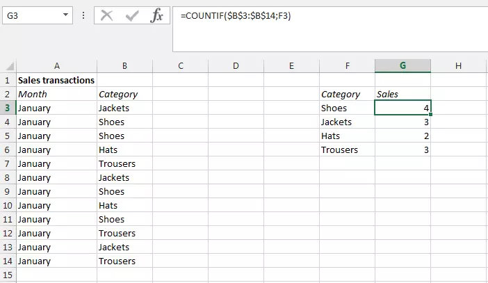
The search criterion can either be given as a value, which you then put in quotation marks (e.g. “shoes”), or by referring to a cell containing this value (e.g. B3). Both entries (range and search criterion) are separated by a semicolon. There are no spaces used in the syntax.
=COUNTIF(B3:B14;"Shoes")
=COUNTIF(B3:B14;F3)
Functions are always introduced in Excel with an equals sign. Otherwise, the program interprets the specification as a simple character sequence and writes it visibly into the cell.
Excel also offers helpful auto completions: simply drag the function (at the bottom right corner of the activated cell) one row further. The specified cells under range and search criterion will be automatically adapted and the function will now refer to cells that are one row lower. If you do not wish for this auto completion and you want the search area to remain the same, you can enter these specifications as absolute values. To do this, insert the dollar sign:
=COUNTIF($B$3:$B$14;F3)
- Free website protection with SSL Wildcard included
- Free private registration for greater privacy
- Free 2 GB email account
The COUNTIF function is not upper and lower case-sensitive.
The COUNTIF function explained with examples
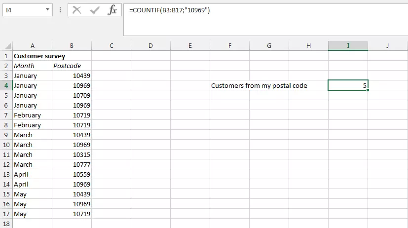
Let’s assume you own a retail store and, for your statistics, you want to find out how many buyers come from your immediate area. To do this, you asked all your customers if they would be willing to provide their postcode. You then enter all your entries one after the other in a table. Now, you can count the cells that contain your postcode.
=COUNTIF(B3:B17;"10969")
In this example we use numbers as text. For the COUNTIF function, in principle, this doesn’t make a difference. But to avoid problems in other situations, you should also format the cells as text.
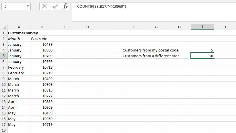
The above example allows you to quickly find out how many customers live nearby your store. On the other hand, if you want to find out how many people live further away, or have a different postcode, you must place a less-than (<) and a greater-than (>) sign before the search criterion.
=COUNTIF(B3:B17;"<>10969")
If you don’t enter the value directly in the function and want to enter the value in a particular cell instead, you need to connect the negation ("<>") with the cell by using the concatenation operator (&):
=COUNTIF(B3:B17;"<>"&B3)
If you’ve asked your customers their age, then these figures have been assigned to the respective postcodes in an extra column. If you think your offer appeals primarily to people over 50, you can verify this assumption with the COUNT IF function. Since you want to include not only all buyers over 50, but also those who are exactly 50, the function must contain the greater-than and equals-to signs:
=COUNTIF(C3:C17;">=50")
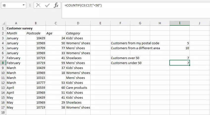
Of course, you will also be interested in the negative result, i.e. how many people are younger than 50. For this, you won’t need a negation: the less-than sign is completely sufficient:
=COUNTIF(C3:C17;"<50")
You can use a similar function in Google Sheets, learn more about the Google Sheets COUNTIF function in our article.
If someone has not entered any information about their age, this value will simply be deducted. You will notice that removing a postcode that is not 10969 will have no effect on the result. To do this, you can extend your formula by counting all cells that are empty and subtracting the number from the first result. In order to tell Excel that you want to use empty cells as search criteria, simply leave the area between the quotation marks empty and write the two characters directly beside each other instead:
=COUNTIF(B3:B17;"<>10969")-COUNTIF(B3:B17;"")
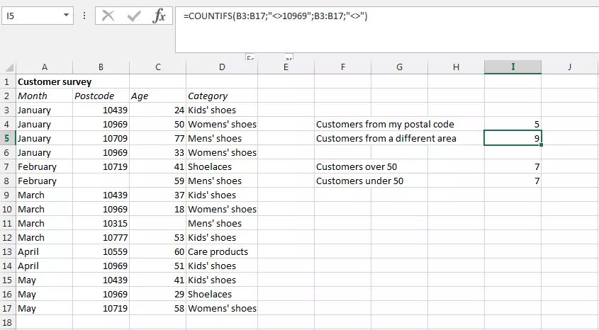
Alternatively, you can also use the extended COUNTIFS function. To do this, add another search criterion to your original formula to specify that empty cells are not to be added. This means that you do not subtract all empty cells, but exclude all empty cells when counting:
=COUNTIF(B3:B17;"<>10969";B3:B17;"<>")
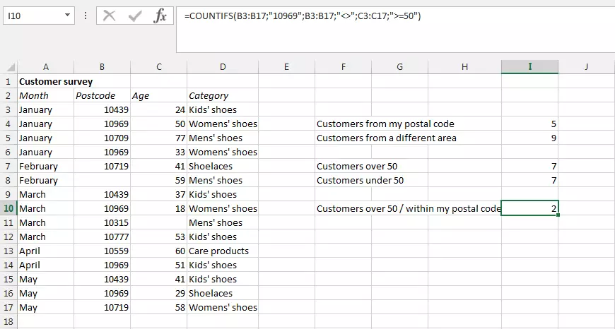
Finally, you can also use the COUNTIFS function to find out – for whatever reason – how many customers over 50 come from your postcode area. To do this, simply insert the additional criterion into the formula:
=COUNTIFS(B3:B17;"10969";B3:B17;"<>";C3:C17;">=50")
Excel has a problem with long strings when using COUNTIF. For search criteria with more than 255 characters you can connect several criteria with the concatenate function "&":
=COUNTIF(B3:B17;"109"&"69").
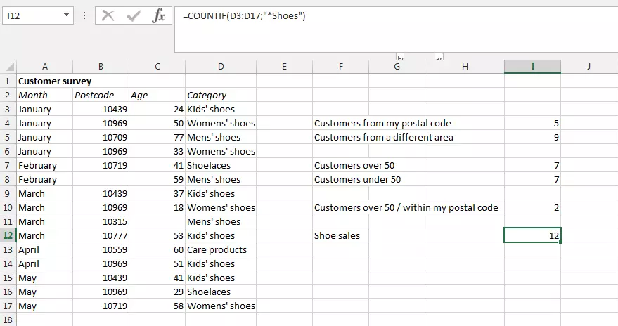
In your customer survey, you also took note of what each customer bought. As the owner of a shoe store, you are interested in how often certain shoes have been sold, and focus on these sales in particular. In this case, you can use a placeholder that can be implemented in Excel with an asterisk (*):
=COUNTIF(D3:D17;"*Shoes")
Placeholders only work for text input. Numerical values cannot be replaced here. The same applies to the question mark (?) as a placeholder: with this, you can replace one character at a time. If you really want to search for a question mark or an asterisk instead, prefix the character with a tilde (~).
- Up to 50 GB Exchange email account
- Outlook Web App and collaboration tools
- Expert support & setup service


