How to wrap text in Google Sheets manually and automatically

You have two options if you want to wrap text in Google Sheets. Although the manual method is very simple, it can often mess up the formatting. Automatic wrapping, on the other hand, always adapts to the formatting, making it the better solution in most cases.

How to wrap text manually in Google Sheets quick guide

1. Double-click the cell
2. Click where you want the break to be in your sentence.
3. Use the key combination [Ctrl] + [Enter] (Windows) or [Cmd] + [Enter] (Mac)

What does text wrapping do?

One of the many similarities between Excel and Google Sheets is that both spreadsheet programs can handle large data sets. However, if the contents of a cell are larger than the allotted space, it often messes up the layout of the spreadsheet.

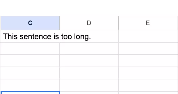
As soon as you start filling in the next cell, some of the information from the previous cell inevitably gets cut off. It’s possible to see the content by double-clicking or viewing it in the formula bar, however, this method is not particularly practical. Let’s take a look at why with the following examples. In the first image, you can see that the information in C1 flows over into D1.

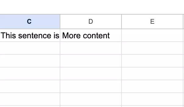
If you now start to write in cell D1, the original text ‘This sentence is too long’ gets cut off and all that’s left of it is ‘This sentence is’.

If you expand the cell so you can see all the content, the entire table can become uneven and end up looking cluttered. The best solution is to use text wrap in your Google spreadsheet. There are several methods for doing this, and we’ll give you tips on what to consider for each one.

How to wrap text manually in Google Sheets

If you only need to wrap text for a single cell in a Google spreadsheet, you can do this manually. To do this, simply follow these steps:

1. Double-click the cell where you want to wrap the text.
2. Now click on the position where you want to wrap the text. The space directly after the last word or number that still fits in the cell is ideal for this.
3. Now press [Ctrl] and [Enter] at the same time if you are using Windows. If you have a Mac, the key combination is [Cmd] and [Enter].
4. The content in the cell will now be cut off at this point, continuing on the next line of the same cell. You can use the text wrap feature as many times as you like in the cell.
5. The last step is to adjust all rows manually so that the document stays organised.

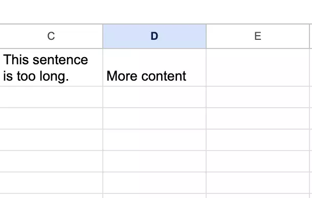
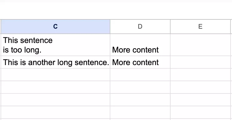
However, the manual method does have a disadvantage. Manual text wrapping is static in Google Sheets, so it doesn’t matter how wide you drag the column, the line break always stays in the same place. This can look unappealing under certain circumstances. Although the information in all the cells is visible, the layout is no longer ideal.

How to wrap text automatically in Google Sheets

Just like with wrapping text in Excel, it’s also possible to do it automatically in Google Sheets. The safest way to do this is to activate it for all cells in your document. The advantage is that the program then structures all content in such a way that it’s still easy to read. At the same time, the formatting stays the same. Below, we’ll explain how to wrap text automatically in Google Sheets:

1. First click the cell that you want to text wrap. If you want to select several cells, hold down the left mouse button and drag the mouse until you’ve covered all relevant cells. If you want to select different cells that are not directly next to or below each other, left-click once, press the [Ctrl] key (Windows) or [Cmd] key (Mac) and then click each cell you want to do text wrapping for.
2. In the bar at the top you’ll find the text wrapping icon. It consists of two vertical lines and a small arrow pointing to the right. When you click on the icon, another small window will open.
3. You have three options to choose from. The current setting is Overflow. Next to it you’ll find the option Wrap. It shows two vertical lines and an arrow that curves to the left. If you click on this, all selected cells will be wrapped automatically.

4. Now, if you change the width of the column, the program will automatically adjust the contents in the cell, ensuring that they always fit perfectly.

5. The third option is Clip. If you select this, the content that exceeds the width of the cell will be removed.

You can also change the setting afterward if you need to. To do this, simply select all the cells again and then click on one of the other two options.