How to merge cells in Excel

Do you have a large data set and want to add headings for a better overview, but don’t know how to go about this? With Excel, you can merge cells, combine columns and join rows with just a few clicks. The spreadsheet program is available in IONOS Microsoft Office Business plans.

Three different ways to merge cells in Excel

In the following steps, use the menu items accessible via the Merge & Center option located in the centre of the Home tab:

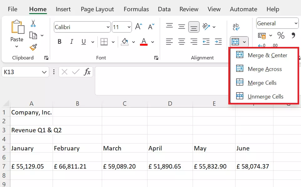
For the following steps, let’s imagine we have a list of monthly revenues for a major company and its branches. The information in the table can be more clearly arranged by adding headings and merging cells.

Method 1: Merge and Center

Let’s assume we want to add a heading with the company name in the row above the data and then merge all the cells together.

Select the cells, columns or rows where you want to insert the heading. You can combine both columns and rows. Click on the Home tab and then select the central button Merge & Center.

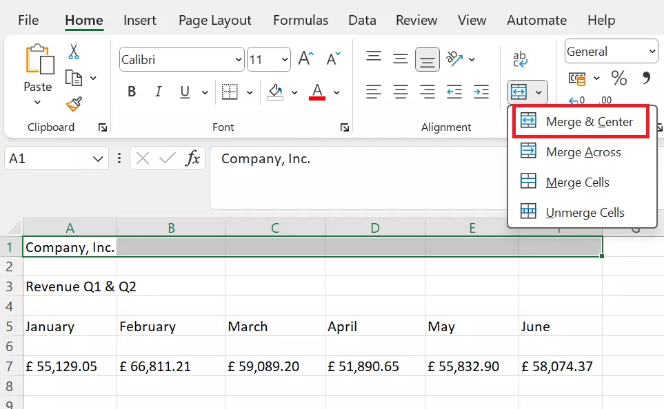
Now, the cells have been combined and the heading has automatically been shifted to the middle of the newly created cell.

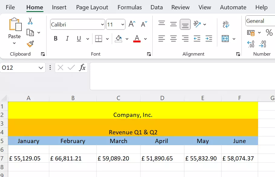
Once you have combined all the desired cells, your table should now be easier to read:

Method 2: Merge Across

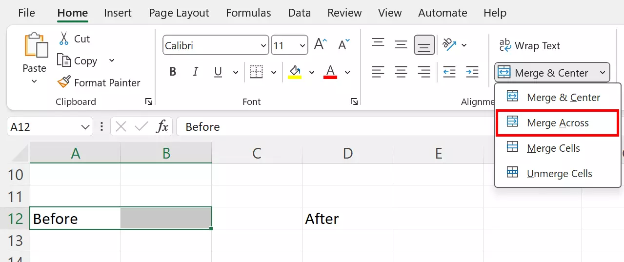
The Merge Across option can also be found under the Home tab. While this allows you to easily combine Excel cells, the function can only be applied across the same row. It can’t be used within the same column, for example.

Method 3: Merge Cells

Excel’s Merge Cells feature works like Merge & Center, just without the centering. Select the cells you want to combine and then click Merge Cells. The text in the original cell will not be automatically centred and will remain left or right-justified.

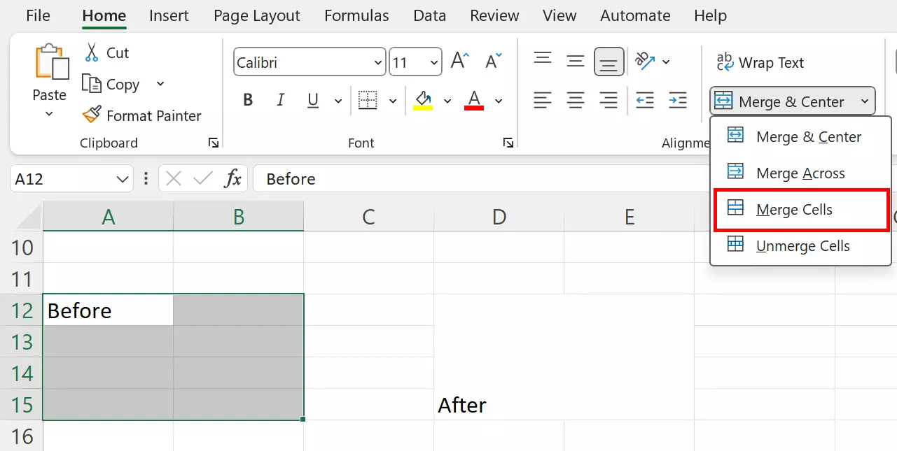
How to unmerge Cells

If you want to split the cells again, select the cells you want to unmerge, and go to Unmerge Cells in the Merge & Center menu.

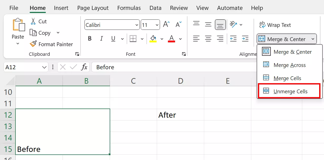
The merged cells will be split. However, text contained in the original cells will not be recovered.

How to combine cells using the ‘&’ sign

Another way to combine cell content into a merged cell is to use the ‘&’ symbol. For instance, if you have separate streets, house numbers and postcodes in a customer list and wish to combine them into merged Excel cells without losing the content of one of the cells, you can simply apply the formula below:

=(cell reference)&(cell reference)&(cell reference)

Step 1: Follow the process above to merge the cells in which you’d like to add content.

Step 2: Move your mouse cursor to the first cell that you want to be combined and enter the formula provided above in order to merge your cell contents into the designated Excel cell.

Step 3: The content will now be combined in a merged cell, but it may look untidy. Add a comma and space to your formula as follows:

=(cell reference)&" "&(cell reference)&", "&(cell reference)

Spaces and punctuation marks (separators) will make the content in the combined cell appear clearer and more structured. Don’t forget to combine each element in the formula with the ‘&’ sign:

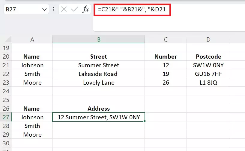
The ampersand is a powerful tool for creating more complex, formatted expressions from individual data entries. This functionality can be used in combination with other Excel formulas to detect errors or generate dynamic content. For example, you could take the example above a step further by using the Excel COUNT function together with the Excel OR function to check the completeness of the address components. In addition, a search function could be created using the Excel MATCH function to make the finished addresses searchable.