How to merge Excel worksheets

Microsoft’s spreadsheet program Excel offers various functions to merge contents from different worksheets. This guide explains step-by-step how to combine worksheets with entries that are identical or different.

How to merge Excel worksheets quick guide

1. Select the cell where you want to merge the data.
2. Click on Data > Consolidate in the ribbon.
3. In the Reference field, select the cells you want to merge and click Add to include them in the references.
4. Click on OK to merge the values.

What are the benefits of merging data in Excel?

The advantage of combining data from different worksheets is that you can create new Excel tables to work with customer or company data. In contrast to the features for merging cells and moving cells, merging data with the Consolidate function or the Power Query Editor allows you to combine data from separate worksheets into one worksheet.

How to merge data in Excel with Consolidate

If you want to merge separate worksheets in Excel, use the Consolidate feature. To use this feature, your Excel file need to have at least two tabs. In the following example, we’ll combine customer data from NYC and LA.

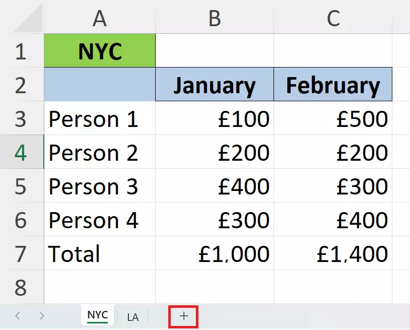
Step 1: Open the file with the worksheets that you want to merge. Click on + next to the worksheet names at the bottom of the window to create the worksheet where the data should be merged. Name the worksheet. A name like ‘Consolidated’ will make it easy to find.

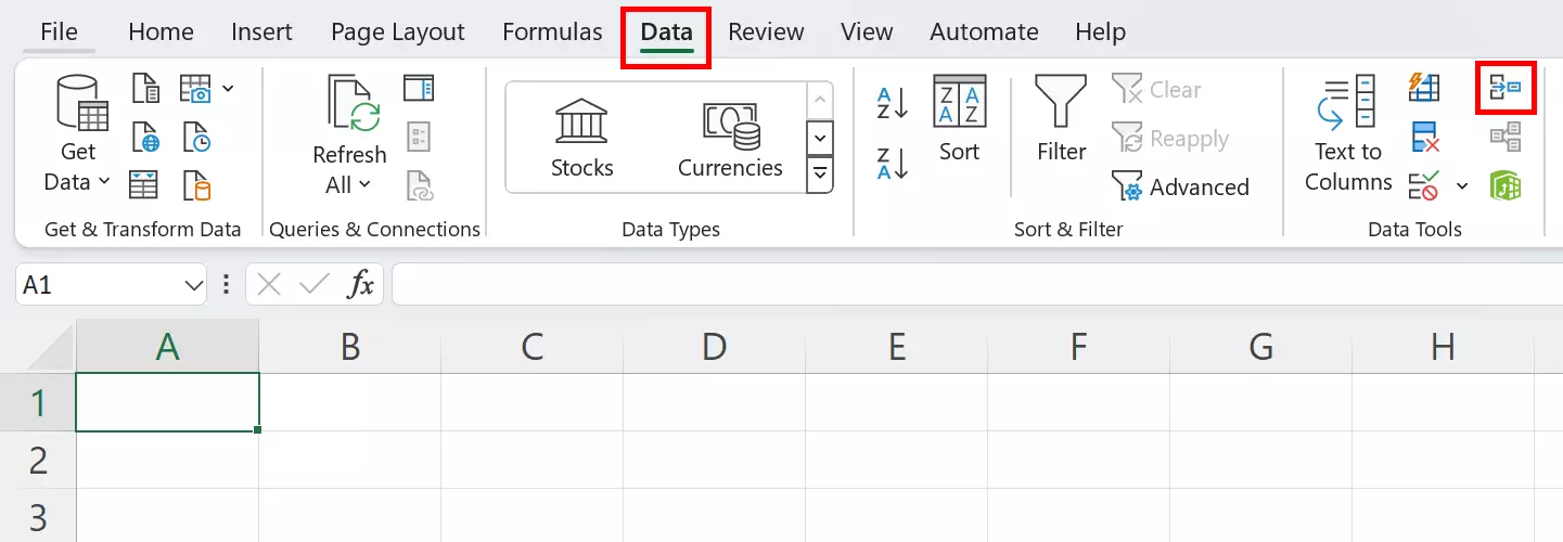
Step 2: In the new worksheet, select the cell where you want to merge the data. In this example, we’ve chosen cell A1. Now click on Data in the menu at the top of the window. In the Data Tools section, select the symbol for Consolidate.

Step 3: The Consolidate menu will open. This is where you can choose how Excel should merge the data (i.e., sum, average, max). In this example, we’ll choose the Sum option so that the values are added together.

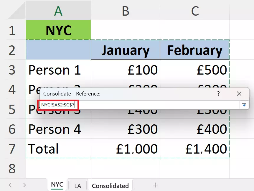
Step 4: Minimise the Consolidate menu by clicking on the arrow under Reference. You’ll now see the menu labelled Consolidate – Reference in its collapsed form.

Step 5: Go to the first worksheet and select the data that you want to merge. You’ll now see the cells you selected in the Consolidate – Reference window. Next, click on the small arrow in Consolidate - Reference.

Step 6: Add the selected reference to All references using the Add button. Repeat the process for the second worksheet.

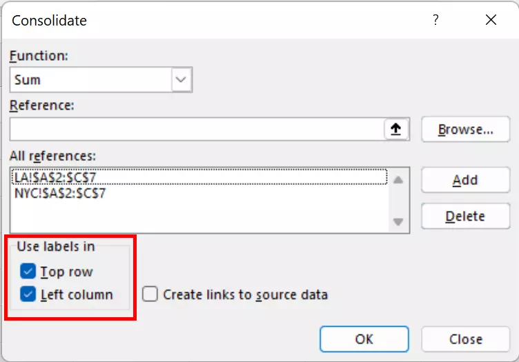
Step 7: Go to the worksheet where you plan to merge the sheets. Click on the tick boxes next to Top row and Left column to ensure the sheet is properly formatted. Then click on OK.

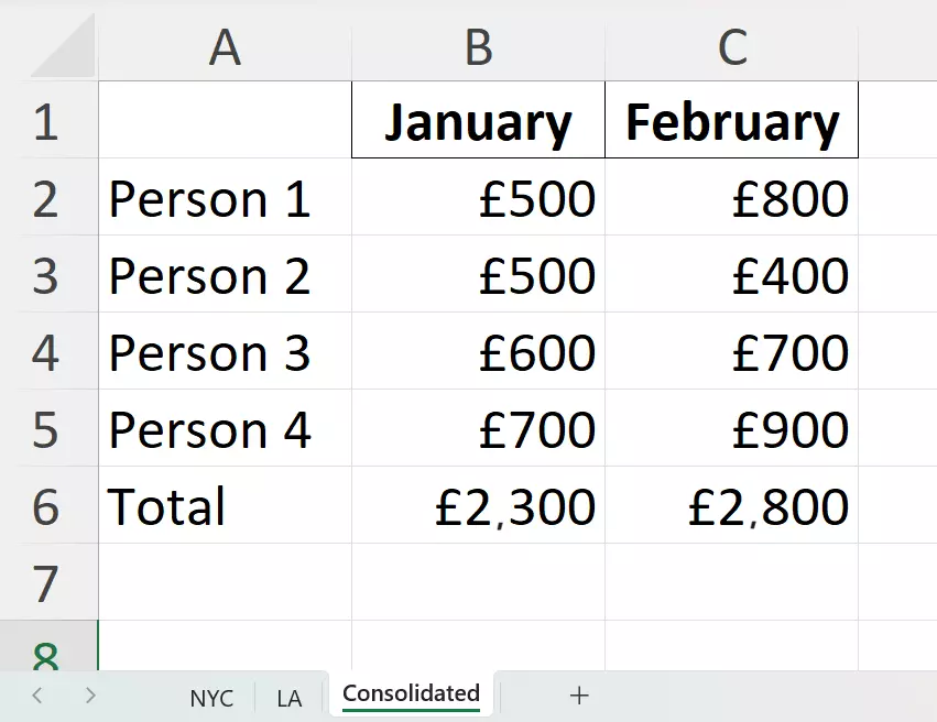
Step 8: You’ll now see the merged data from the other Excel sheets in the new worksheet.

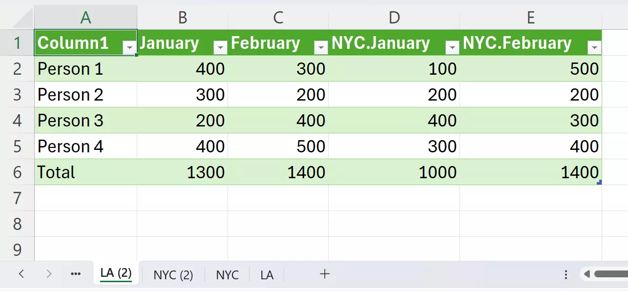
How to merge data in Excel with the Power Query Editor

For simple merging operations where both worksheets have the same formatting and information, the consolidation feature will suffice. However, if you want to merge sheets that contain, for example, different values for the same customer group, the Power Query Editor is your best bet.

Step 1: Go to the first worksheet and select the contents. Then click on the Data menu and afterwards on From Table/Range. After the Create Table window pops up, click OK.

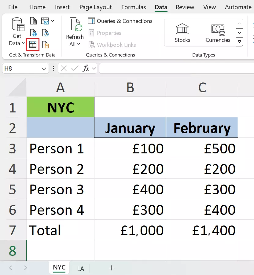
Step 2: The Power Query Editor will now open with the contents of the table you selected. To add the contents of the second table, click on New Source in the upper right-hand corner of the Excel window. Select File and then Excel Workbook.

Step 3: Import the Excel file containing the second table and click OK in the navigator that opens.

Step 4: Click on Merge Queries and then again in the dropdown menu.

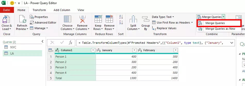
Step 5: A window labelled Merge will open. Select the two tables and choose the columns with the same data to ensure consistent formatting.

Step 6: To make the contents of the table visible, click on the arrow symbol under Table 2 and untick the boxes next to the columns with the same data (in this case Column1). Tick the boxes for different data that should be added.

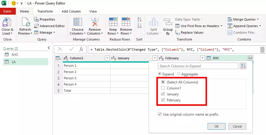
Step 7: The editor will then merge the contents you selected into a single table. Click on Close & Load to place the merged table in a new Excel worksheet.