How to use VLOOKUP in Google Sheets
VLOOKUP searches a column from top to bottom for the values you’re looking for. Even in huge directories, the vertical lookup function allows you to quickly find the information you need. The following article explains how to do VLOOKUP in Google Sheets and provides helpful examples as well.
What is VLOOKUP?
Spreadsheet programs offer users many benefits for working fast and effectively with spreadsheets. If you use spreadsheets regularly, you’re no doubt already familiar with the range of practical functions that make working with Excel or Google Sheets more efficient and convenient. VLOOKUP is one such function – enabling you to find information and values in huge directories and spreadsheets in no time at all. But how exactly do you use VLOOKUP in Google Sheets?
The function can also be used in Microsoft’s well-known spreadsheet program. VLOOKUP in Excel works similarly to how it does in Google Sheets.
Let’s assume you have a massive directory with customer names, numbers and addresses. Each customer entry is assigned to a column, and the product category that the customer most frequently orders from is also included. A phone call has been scheduled with a person listed in the directory and you want to quickly find out which product category they are assigned to. Using the customer number and VLOOKUP in Google Sheets, you can find the value for the search term, without having to go through the entire list manually for the information you need.
- Familiar Google tools all in one place
- Using Gmail with your domain from IONOS
- Configure business Gmail for your domain
What is the syntax for VLOOKUP in Google Sheets?
Like with any other function, it’s important to fill out VLOOKUP correctly. If the formula contains errors, Google Sheets will not be able to properly run the search. The VLOOKUP formula looks like this:
=VLOOKUP(search_key, range, index, [is_sorted])The search_key is the first value you’re looking for. In range, you define the table or area in the spreadsheet that should be searched. Index refers to the column that contains the return value of your search. The index is expressed as a number and represents the position of the column that will be searched relative to the column where the search key is located. If your search key is located in column C and you’re looking for a corresponding value in column F, the index will need to be 4. This is because if you start counting from 1 with column C, column F will be the fourth column.
If you are using Google Sheets in a language other than English, it doesn’t make a difference if you enter the term ‘VLOOKUP’ or the equivalent term for this function in another language. Depending on the language settings in your Google account, the software will automatically change the names of the functions in Google Sheets.
The optional formula suffix [is_sorted] defines whether the column to be searched is sorted or not. If the column isn’t sorted, you should enter ‘FALSE’; otherwise enter ‘TRUE’. If the parameter is left empty, Google Sheets will automatically set it to ‘TRUE’. Even though the parameter is optional, it still plays a decisive role in the outcome:
- FALSE: The function searches for an exact match and returns the first result found.
- TRUE: The function doesn’t search for an exact match, but instead returns the value that’s closest to the search key.
Here’s an example of the VLOOKUP formula in Google Sheets:
=VLOOKUP(A10,A2:C10,3,FALSE)This formula instructs Google Sheets to run a vertical search in a column that’s three columns away from column A. The cells between A2 and C10 are searched. The search value is entered in cell A10. Google Sheets then outputs the corresponding value in column C.
Looking for a modern office solution for your company? The Google Workspace solution from IONOS offers you many benefits, such as personalised email domains and 30 GB of online storage for each of your team members. With IONOS, you also benefit from prioritised Google support.
Step-by-step examples for using VLOOKUP in Google Sheets
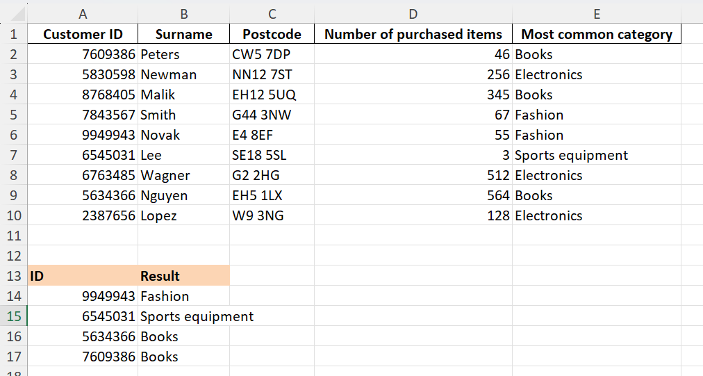
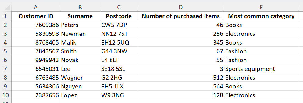
The following example of VLOOKUP in Google Sheets should help to give you a better idea of how the function works. We’ll use the following table as our initial dataset:
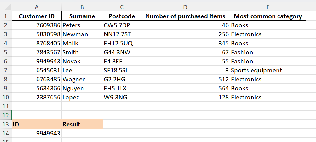
Step 1: Add the area you want to use for your search query and the result anywhere below or next to the table in your spreadsheet. You can simply enter ID and Result as headings if you like. In the field for the Search key, enter the cell value that you want to search for.
Step 2: Enter the formula for VLOOKUP in the field where you want to see the search result. In our example, we’ve chosen the field B14. Enter the following formula there:
=VLOOKUP(A14,$A$2:$E$10,5,FALSE)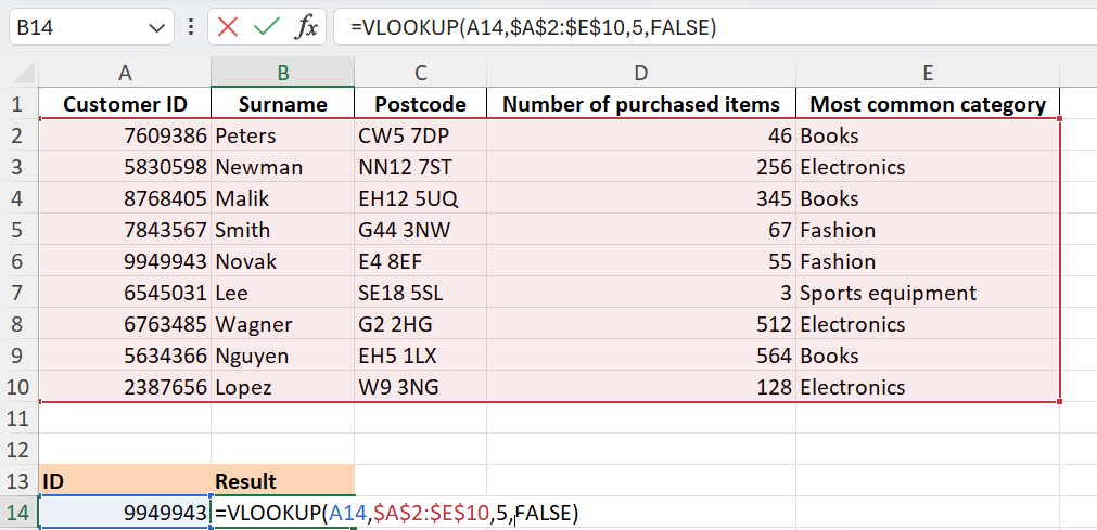
Step 3: You’ll now see the result Fashion in the field where you entered the VLOOKUP formula.
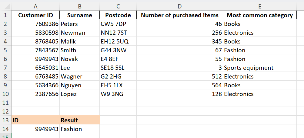
Step 4: You can now enter the different customer numbers from column A as search keys. You can change the search key in the VLOOKUP formulas for the different customer IDs manually or simply click on field B14, which contains the category Fashion, and drag the blue square down to the other cells. The formula will automatically be adopted, and you’ll get the results you’re looking for.
