Excel SUM function
The Excel spreadsheet can be used to create presentable tables and diagrams based on them, and also to carry out simple and complex mathematical calculations. You can calculate results of ordinary formulas as well as specific functions. The latter are particularly advantageous if the calculation is extensive and includes many values. The Excel SUM function allows the fast addition of several cell values, which the software does by immediately adjusting the total when the numbers in the affected cells change. This article explains how to use the SUM function in Excel and what to keep in mind.
- Up to 50 GB Exchange email account
- Outlook Web App and collaboration tools
- Expert support & setup service
Excel SUM Function: The Most Important Key Data at a Glance
Before we illustrate the functionality of the Excel SUM function by means of a specific example, first the conditions linked to its use need to be clarified – above all, the syntactic rules, without which the use of the function is not possible. However, these are not too complicated in the case of the Excel SUM function, as Excel is only informed of the relevant values and has to add these together to provide the appropriate return value. The syntax looks like this:
=SUM(Parameter1;Parameter2;…)SUM requires at least one parameter. “Parameter1” is mandatory, while “Parameter2” and all others are optional. Overall, the function can process up to 255 individual parameters, whereby a parameter can refer to the following:
- a value like “4”
- a cell reference like “D4”
- a cell range like “D4:F8”
The important thing is always the separation by semicolon which signals to Excel the start of a new parameter.
With the preceding equals sign, Excel recognises that there is a formula in the cell itself. It must be used for Excel functions such as “SUM” to work.
Excel: Calculating the Sum via Function
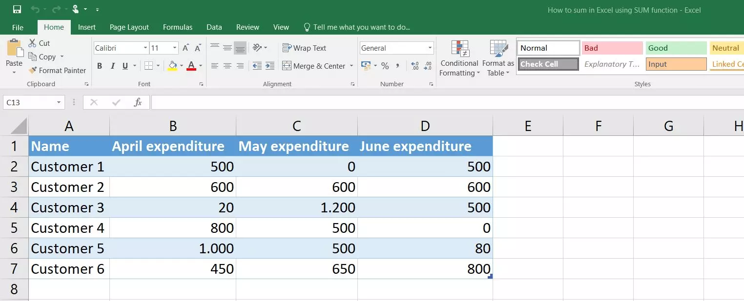
As already mentioned, the use of the Excel SUM function is particularly practical if you want to add up several values. The only requirement is that you have already stored these values in separate cells in an Excel document. In the following, we will use a data set as the basis for the following instructions, which contains the monthly expenditure in the period from April to June of six different customers as an example:
Example Scenario 1: Calculate the Total Expenditure of Individual Customers (Data in the Same Row)
A first possible application case for the Excel SUM function is the addition of the monthly purchases that a single customer has made in the three months. To do this, first select the cell in which the return value of the function should be shown – i.e. the total expenditure of the desired customer. Then paste the following content into that cell:
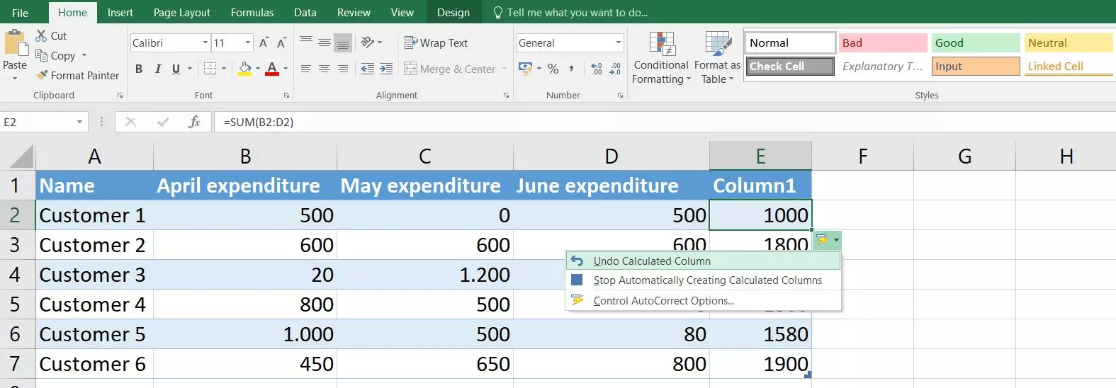
=SUM(B2:D2)Press Enter to confirm the function. If you work with a data set that is not formatted as a table, you will get the return value for the expenditures of Customer 1 that are behind the distinguished cell range "B2:D2". In the case of a formatted table, Excel transfers the SUM function to the entire column, so that it also presents the monthly expenditures of the other customers:
If the automatic transfer of the function to the entire column is not desired, it can be easily undone: Click on the button “AutoCorrect feature” on the original cell and select “Undo Calculated Column”. Here, you can also disable the automatic creation of such “calculated” columns completely.
You can also select the fields that should be processed by the Excel SUM function by mouse, after opening the bracket in the formula. Simply click on the first Excel cell, keep the left mouse button pressed, and then move the cursor over all other fields that should be included in the calculation.
Example Scenario 2: Calculate the Total Expenditure of All Customers for a Specific Month (Data in the Same Column)
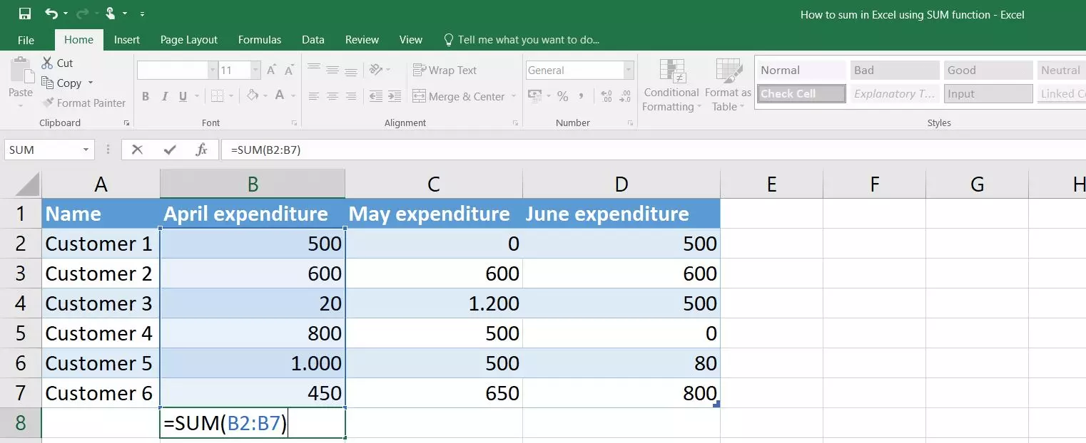
Just as the Excel SUM function can be applied to all values in a row, it can also be applied to a specific column. With the example data set, this means that you can receive the total value of common expenditures of all six customers in April, May or June. Initially, you again have to select a free cell – then the total for April is calculated by, for example, the following formula:
=SUM(B2:B7)With a formatted table, the result, which you can get after confirming the formula using the Enter key, can optionally be incorporated as part of the table result row, as an ordinary table row or in an independent row under the table – without its own formatting. Click on the already covered AutoCorrect function and select the desired option:
Example Scenario 3: Calculate the Total of All Expenditures (Multi-Column and Row Data)
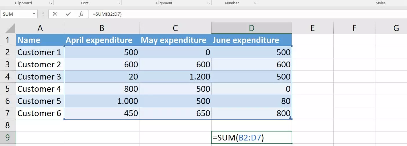
The Excel SUM function can not only be applied to a single row or column, but also to add up the values of cells across many rows and columns. This way you can easily get an overview of the total expenditures of the six customers of the example data set in the three months listed:
=SUM(B2:D7)In this case, press Enter again to activate the formula.
Example Scenario 4: Sum of Total Expenditures for a Specific Customer Group (Data in Non-Adjoining Cells)
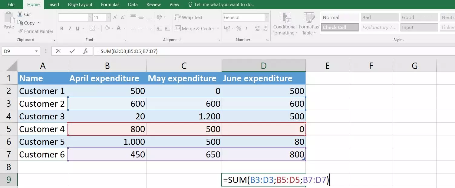
In the previous examples of the Excel SUM function, only one parameter was needed at a time, as the relevant cells were adjoining in all cases. As already mentioned, however, you can use up to 255 different parameters in SUM formulas in principle which allows Excel to solve calculations related to cells or ranges of cells that are not adjacent. For example, in the tutorial spreadsheet, we can segment customers and determine how much Customer 2, Customer 4, and Customer 6 have jointly spent from April to June:
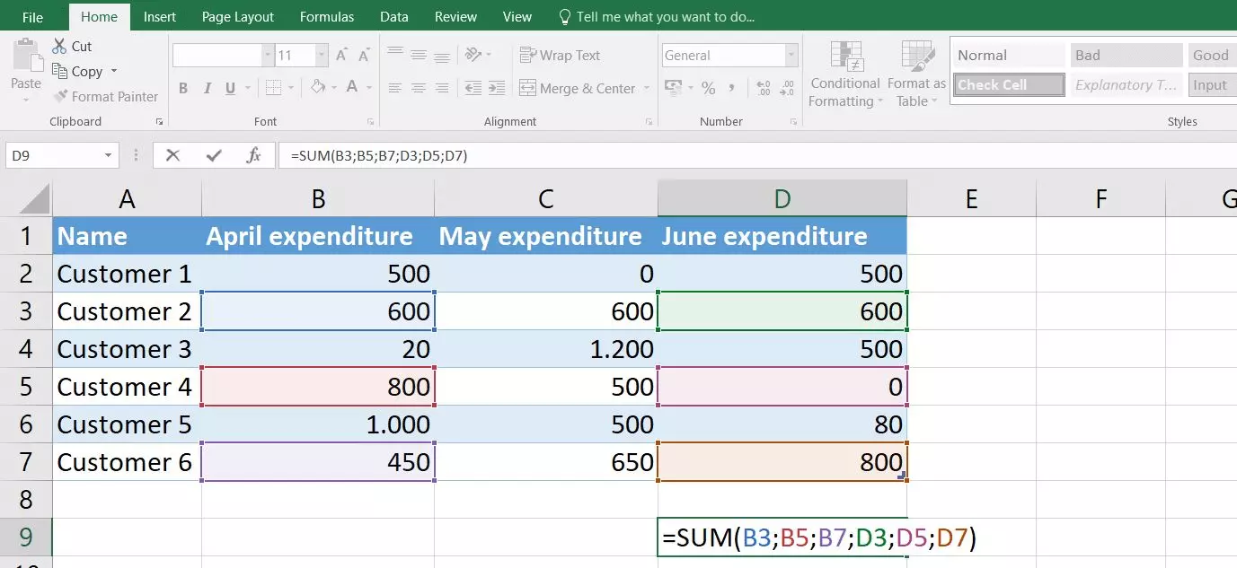
=SUM(B3:D3;B5:D5;B7:D7)The formula becomes even more complex if the expenditures in May are disregarded and only the months of April and June should be evaluated. In this case, instead of three cell range parameters, six cell reference parameters are needed:
=SUM(B3;B5;B7;D3;D5;D7)Even with non-adjoining cells, you can select the fields to be processed by mouse. In this case you have to press the [Ctrl] key instead of the left mouse button. When holding down the key, simply click on the desired cells in sequence by left clicking, and Excel will add them to the SUM formula.
- Up to 50 GB Exchange email account
- Outlook Web App and collaboration tools
- Expert support & setup service


