Excel AND function: step-by-step instructions and examples
The popular spreadsheet program Excel included in Microsoft Office allows you to enter numbers and text in spreadsheets to make sense of your data. Excel offers a wide range of functions which have a variety of uses, especially for worksheets containing multiple values. With over 400 different options, you can edit or evaluate your data automatically. Excel AND has always been one of the most popular functions. Using this function, you can define up to 255 conditions and check whether the values in your spreadsheet meet these conditions in just a few clicks. In the following, we will provide you with step-by-step instructions on how to use the Excel AND function.
Excel AND function – TRUE or FALSE?
Excel AND is one of Excel’s logical functions which allows you to check whether or not certain conditions have been met. This function results in two possible return values: if all the conditions you specified have been met, Excel will output the return value “TRUE”, but if even one condition has not been met, the return value will be “FALSE”.
Excel AND: a step-by-step explanation of how to use this function
So, you have an Excel spreadsheet containing a many values, and you wish to determine which values meet specific requirements. Performing a manual search would take a lot of time. Not to mention, the human eye can easily overlook values and is thus a possible source of error. That is why Excel provides the AND function which is great for automatically checking whether certain conditions have been met. In the following, you will find step-by-step instructions on how to use the Excel AND function.
Step 1: Defining conditions
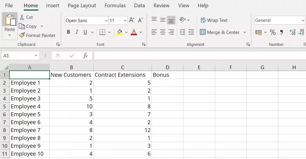
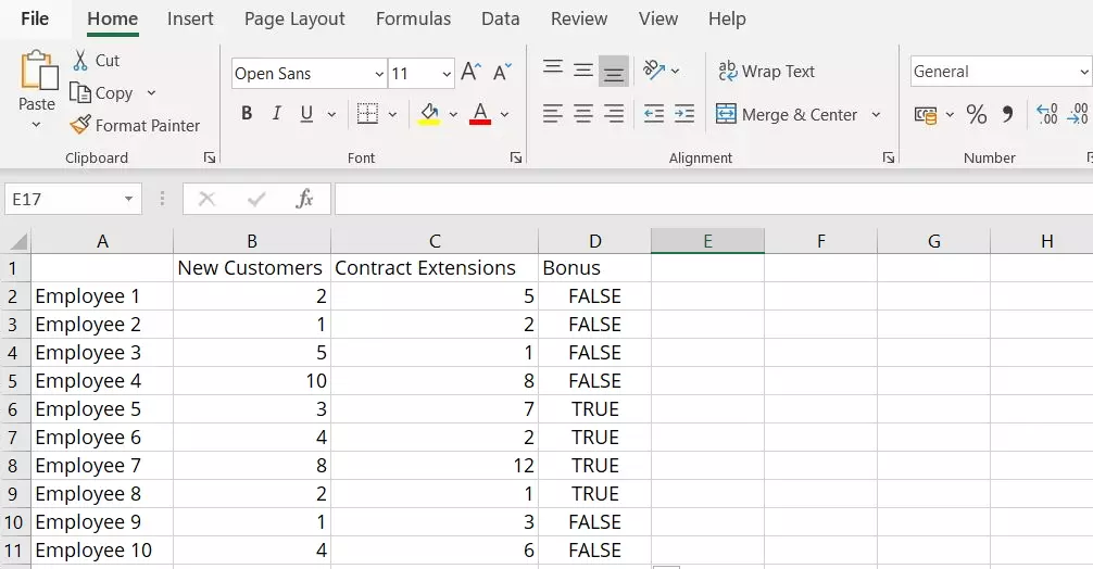
In this example, we will check which employees meet all the requirements for receiving a bonus payment. There are two conditions: the employee must have obtained at least three new customers and two or more contract extensions. So, for example, if an employee has obtained five new customers (i.e. more than required) but only one contract extension, they will not receive a bonus. The Excel AND function works well for this concrete example because it allows the program to optimally test whether all the conditions have been met.
Step 2: Using the Excel AND function
After entering all the values for this Excel AND example, you apply the function to the spreadsheet. For clarity’s sake, it is recommended to use a separate column for the function and its return value. There are two ways to enter the function:
Enter the function in the cell
You can enter the function in the cell where you want the return value to be displayed. Functions always begin with an equals sign and the name of the function. This is followed by the individually defined parameters for the function which are placed inside parentheses.
The following is the general syntax for the Excel AND function:
=AND([logical1];[logical2];etc.)If you use lowercase letters when writing “AND”, Excel will automatically correct the input. Therefore, you do not need to worry about using the correct capitalisation.
The logical values are your conditions which are separated with a comma or semicolon depending Excel version you are using. When using Excel AND, you can enter anywhere from two to 255 conditions in the program. However, you should avoid using an excessive number of conditions. The more conditions a function contains, the more complex and nested it becomes. This makes it more difficult to create, check, and manage a function.
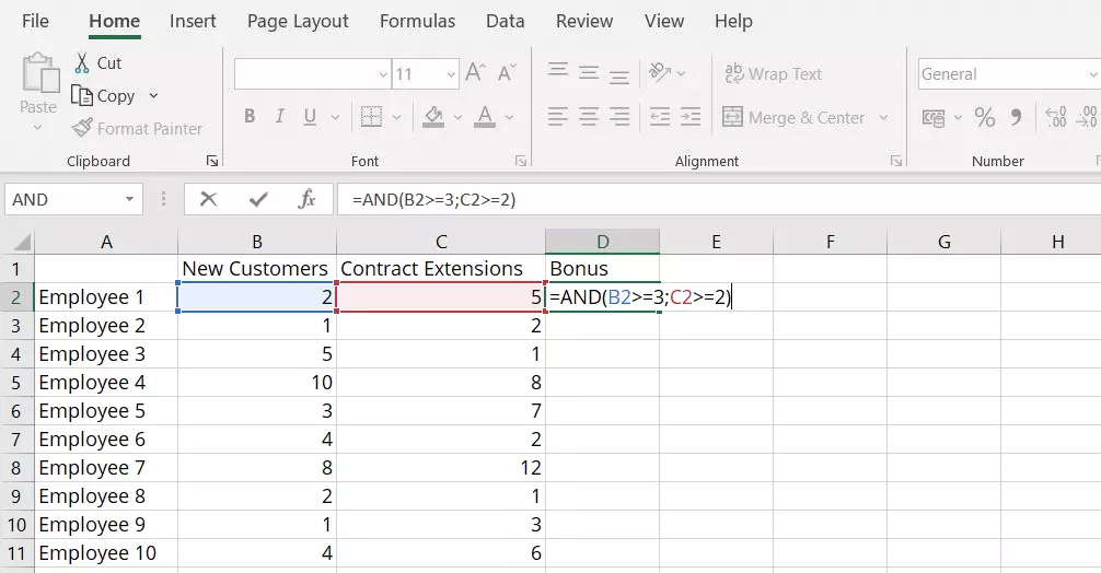
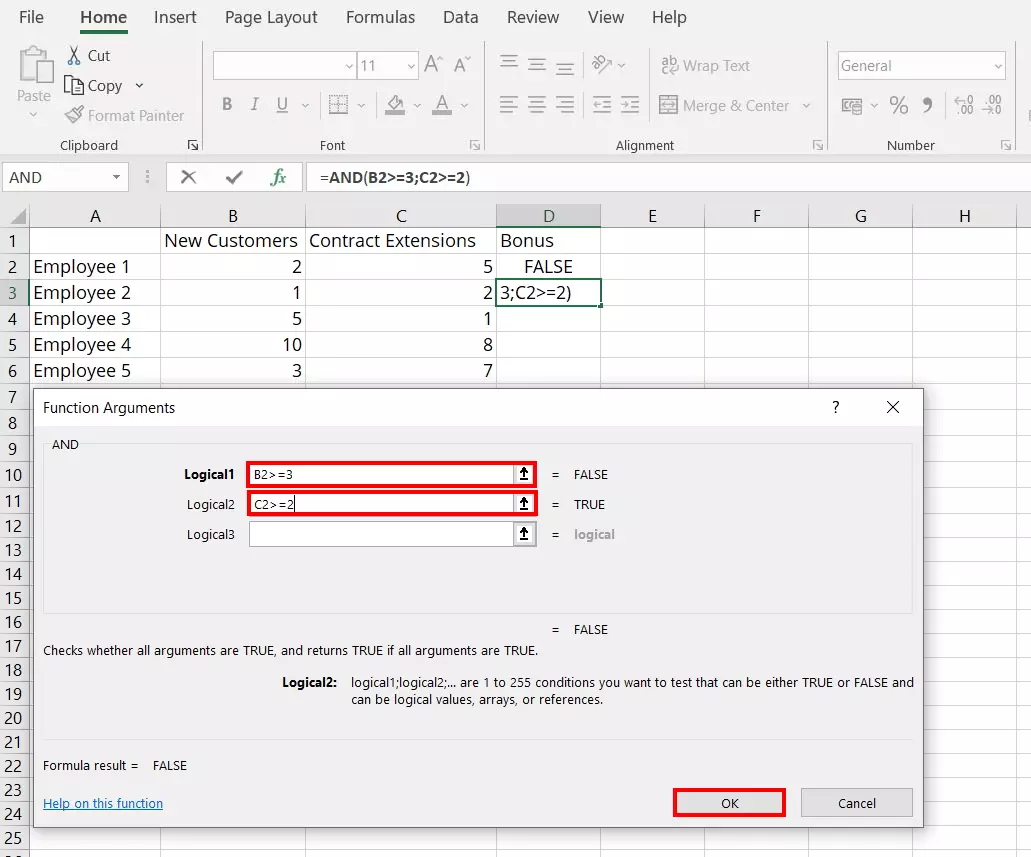
When defining and entering the logical values (i.e. the conditions), use the equals sign (=), greater-than sign (>) and less-than sign (<). In our example, logical value 1 is the condition stating that an employee must have obtained at least three new customers. The value in column B must therefore be greater than or equal to three. You define this condition by entering “B2>=3”. Logical value 2 is the condition stating that the employee must have also obtained two contract extensions. This is defined by entering “C2>=2”. In our example, the entire Excel function is as follows:
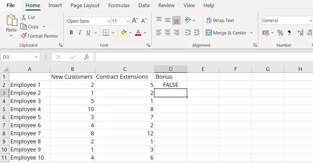
=AND(B2>=3;C2>=2)Press the Enter key on your keyboard to confirm your entry. Excel will then display the resulting return value in the cell, not the function. In our example, Employee 1 only meets one of the two conditions. Therefore, the displayed return value is “FALSE”.
Open the function using the menu
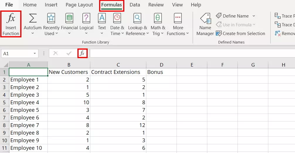
Alternatively, Excel offers the option to use a separate dialogue box for the Excel AND function. To open this dialogue box, go to “Formulas” and then select “Insert Function” in the menu or left-click on the corresponding icon located next to the formula bar.
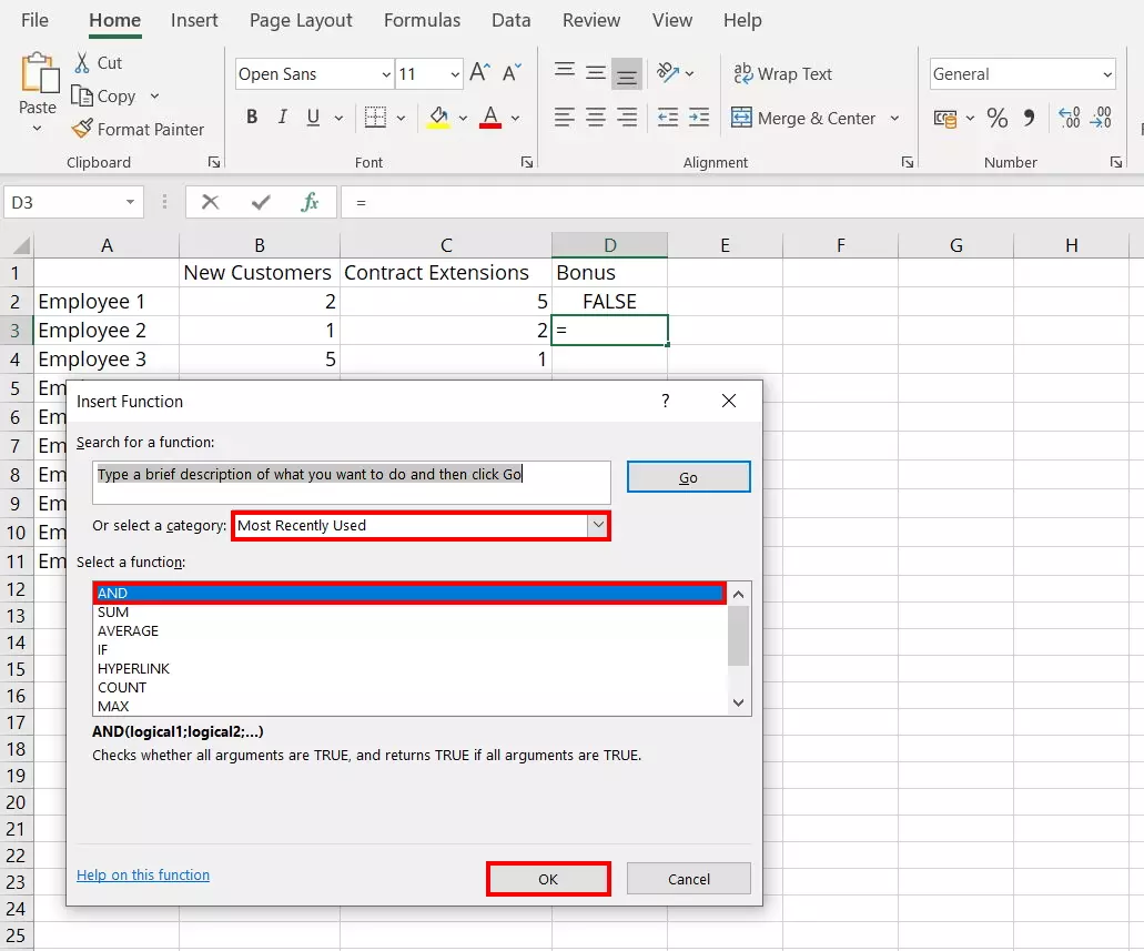
Excel will then open the “Insert Function” dialogue box. When it opens, the category “Most Recently Used” will automatically be selected. If you have recently used the Excel AND function, it will appear in the list below. If this is the case, select the “AND” function. This will highlight it in blue. Confirm your selection by clicking “OK”.
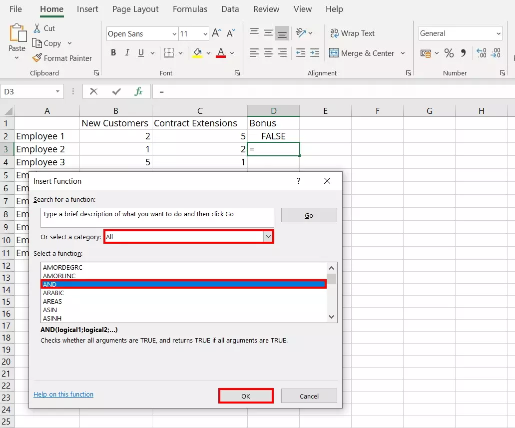
If the desired function is not included in the list, open the drop-down menu next to “Or select a category” and select “All”. Excel will then display a list of all the available functions. Use the arrows to scroll until you find the “AND” option. Left-click on the function. Once it is highlighted blue, confirm your selection by clicking “OK”.
Excel will then open the “Function Arguments” dialogue box. In this dialogue box, you enter each condition on a separate line. As you do this, the program will already display whether the conditions have been met. Once you have entered all the conditions, confirm them by left-clicking on “OK”. Excel then applies the formula and displays the resulting return value in the cell.
Step 3: Checking all the spreadsheet values
You do not need to manually insert the Excel AND function in each row. If the defined conditions apply to all values (all employees in our example), Excel can apply the function to all lines in just a few clicks.
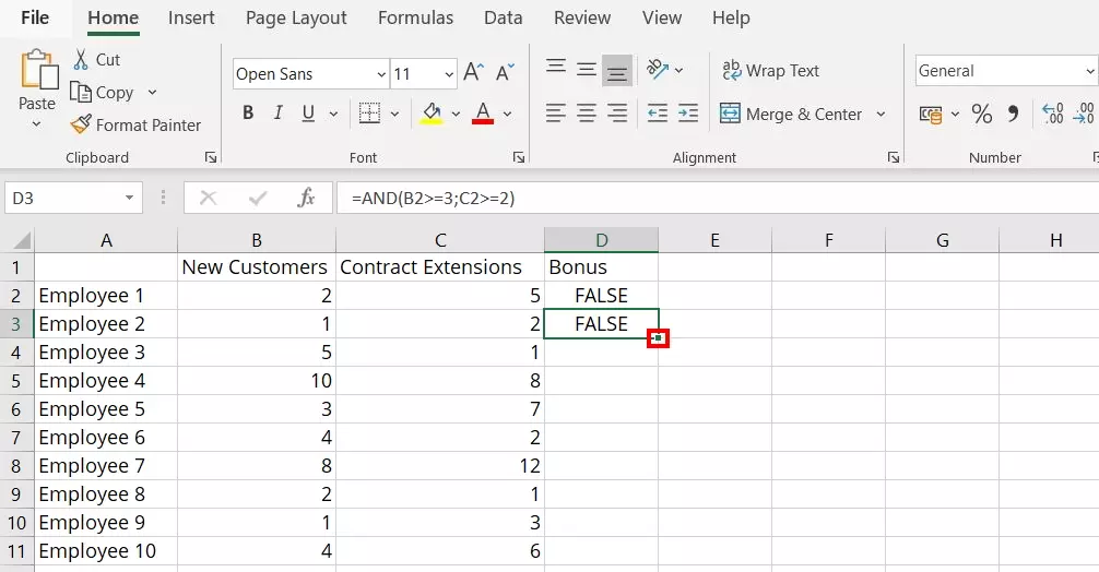
To do this, first select the cell containing the AND function by left-clicking on it. Then, left-click on the corner of the green rectangle around the cell. Keep holding the mouse button and drag the function across all the cells where it is to be applied. In our example, this includes cells D2 (Employee 1) to D11 (Employee 10).
Comparing expected and actual values using the IF function
Using the IF function, you can check whether a requested value matches an expected one. The general syntax for this formula is as follows:
=IF(logical_test;[value_if_true];[value_if_false])The IF function is very similar to the AND function. The following are the two main differences:
- The IF function only checks if one of the conditions has been met.
- You can individually define the displayed return values for the evaluation when using the IF function.
When using the Excel AND function, the possible resulting return values are “TRUE” and “FALSE”. In contrast, when using the IF function, you use the parameters “value_if_true” and “value_if_false” to define the resulting return values that Excel displays in the cell after the evaluation.
The special SUMIF function can be used to add only specific values together. You can read about how to use this function in our article “The SUMIF function explained”.
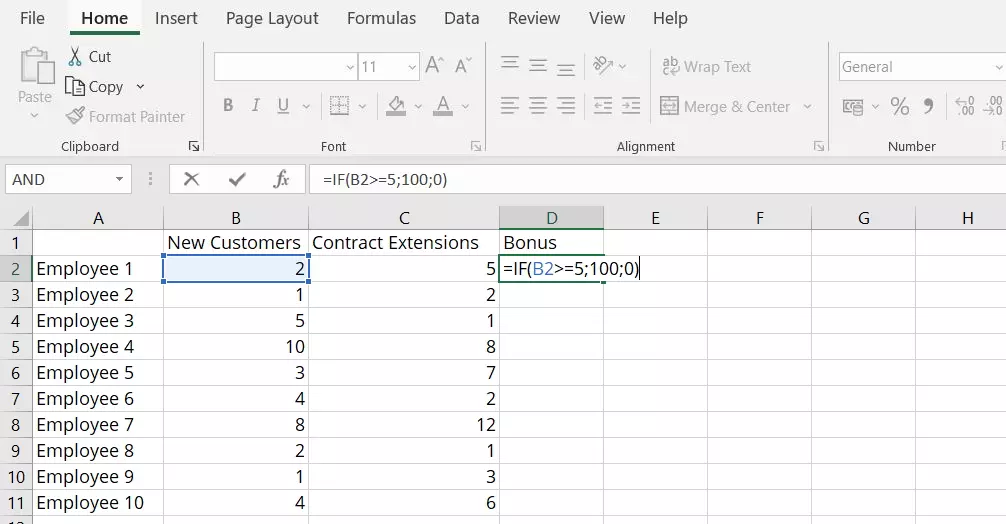
In our example spreadsheet, the IF function is used as follows: If an employee obtains at least five new customers, they will receive a bonus of 100 euros. If the employee does not achieve this target number, their bonus will be 0 euros. This condition is defined by the following IF function:
=IF(B2>=5;100;0)Combining the Excel AND function with the IF function
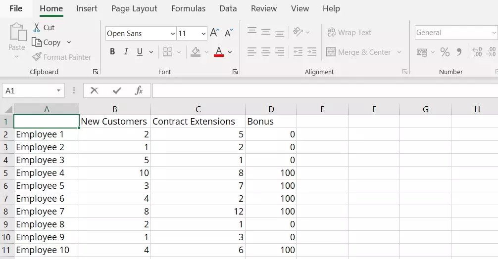
Excel allows you to combine multiple functions in the same formula. Combining the AND and IF functions provides two advantages: you can define multiple conditions and individually define what the displayed return values will be.
When you combine the two functions, the general syntax will look like the following:
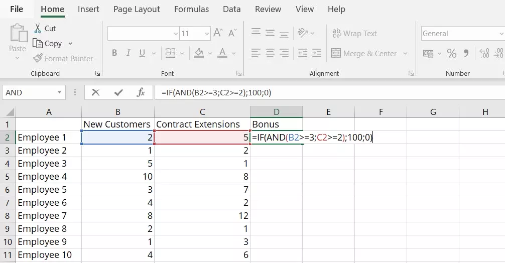
=IF(AND([logical1];[logical2];[logical3];etc.);[value_if_true];[value_if_false])For our example, the formula would look like this in practice:
=IF(AND(B2>=3;C2>=2);100;0)

