How to edit drop-down lists in Excel

Theoretically, once you create a drop-down list in Excel, it can be used indefinitely. That said, at some point, you may wonder ‘How do I edit a drop-down list in Excel?’. We explain what options you have for editing drop-down lists.

Step-by-step instructions for editing drop-down lists in Excel

Every drop-down list in Excel requires you to compile a list of the entries in the same workbook. This list should ideally be formatted as a table so that when you change the entry in a table cell, this change is immediately visible in the linked drop-down list. It is a different matter when you want to insert or delete cells. For these changes to also be visible in the drop-down list, the linked area has to be adapted.

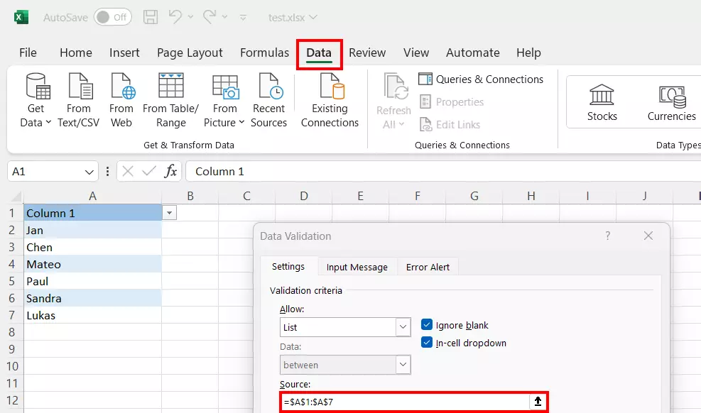
To do this, select the cell (or cells) using the drop-down function and then follow these steps:

1. Go to Data Validation in the Data menu.
2. Under Source, reconfigure the area for your drop-down list. You can do this by either directly typing in the new reference or highlighting it using the select function.
3. The changes will then also be visible in the drop-down list.

How to change error alerts and input messages in Excel drop-down lists

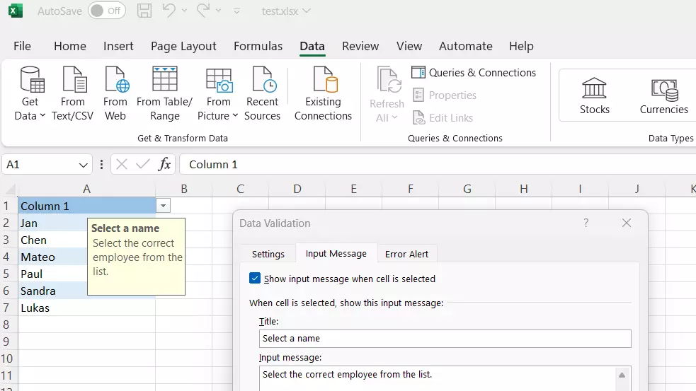
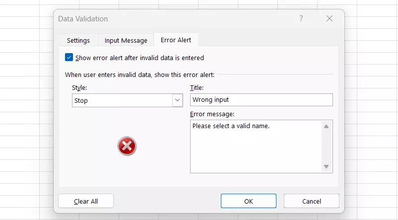
Data Validation provides even more options for editing drop-down lists in Excel. Simply click on the other tabs in the Data Validation section:

Input Message: The input message feature allows you to make comments. This is especially important if third parties will be working with the file. You can use a comment to explain how to properly use the file in detail or give more information about the drop-down list. If the user clicks on the cell with the drop-down list, the comment appears in a yellow box.

Error Alert: The error alert menu gives you the possibility to provide feedback on incorrect entries. In principle, a drop-down list prevents invalid entries from being used because users are meant to select the value they want from the list. However, other entries that are not on the list can be made through the formula bar. If a value is written in the row and is not in the list, an error will occur. The error alert gives you the option of explaining to other users what the correct procedure is to follow. You can also choose from three different types of error alert:

• Stop: This style of error alert is displayed, and the incorrect entry is not permitted.
• Warning: A warning error alert is displayed, and the user is given the option to allow or undo the error.
• Information: This type of error alert is displayed, and the incorrect entry is adopted in the cell anyway.

How to adapt the appearance of drop-down lists in Excel

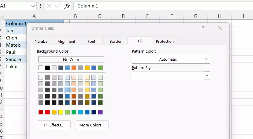
The appearance of drop-down lists in Excel can also be adapted. Like with any other cell, you start by right-clicking the cell containing the drop-down list. Then select Format Cells in the context menu. Here, you can adapt the cell’s appearance:

• Number: If your drop-down list should include numbers, you can change how these are displayed.
• Alignment: If the text isn’t going to be aligned horizontally, this option lets you change the alignment and direction of the text.
• Font: The font, font style and font size can be adapted in this menu item.
• Border: If you want to make the drop-down list stand out with a border, you can change the size and appearance of the line here.
• Fill: Filling the cell with a colour of your choice is another way you can draw attention to it.