How to add a drop-down list in Google Sheets
If you prefer not to manually enter the attributes of a value into the corresponding cell in Google Sheets each time, you can utilise drop-down lists. These lists allow you to select from predefined attributes. Below, we explain how to create drop-down lists in Google Sheets.
- Our experts run your campaign
- Increase your online visibility
- Save money thanks to greater efficiency
Why are drop-down lists so useful in Google Sheets?
If a cell contains a drop-down list in Google Sheets, users can select a value from a pre-defined list with just one click. The selected value is then displayed in the cell. Selecting an existing value is much easier than having to type the value manually. Drop-down lists also help keep your data accurate and consistent. If multiple people are working on the same spreadsheet, using drop-down lists means that only accepted values are possible. This results in fewer typos and greater time savings which are among the many good reasons for using drop-down lists in Google Sheets.
Discover the key differences between Google Sheets and Microsoft Excel in our comprehensive comparison article: Google Sheets vs Excel.
How to create drop-down lists in Google Sheets step by step
Google has made it as easy as possible for users to add drop-down lists to individual cells. To add a drop-down list, follow the steps below:
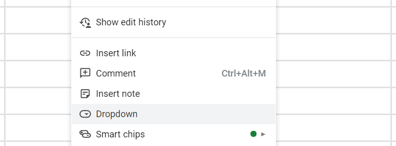
Step 1: Choose a cell, then right-click and select Dropdown:
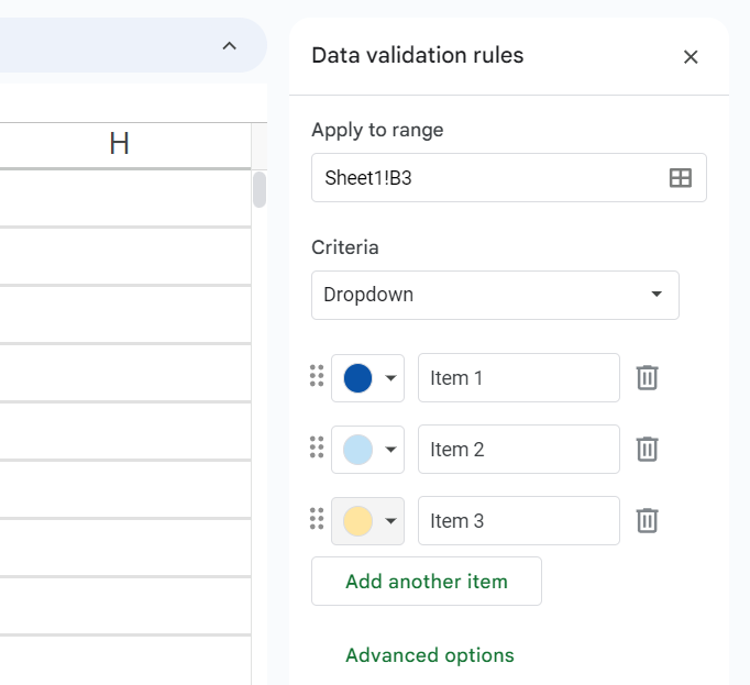
Step 2: Enter all the desired elements of the drop-down list manually under Criteria. In addition to choosing a unique name, you can also assign an individual colour to each element. To confirm the values, click on Done:
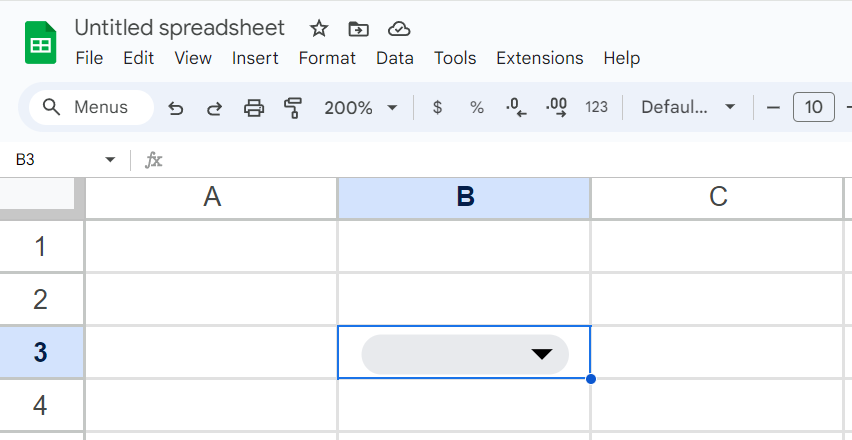
Step 3: A drop-down list has been added to the cell you selected. You can confirm this by checking for the downward arrow in the cell:
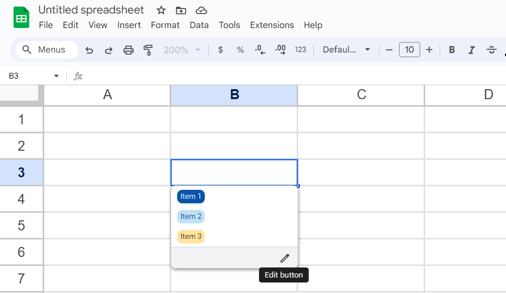
Step 4: Click on the arrow to open the drop-down list in the cell. Check whether the elements are listed in the desired order and are spelled correctly. If you want to make changes, click on the Edit button option.
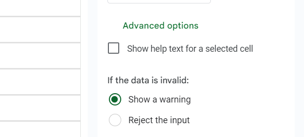
Step 5: Do you want to add a warning to your Google Sheets drop-down list to alert users when an invalid value has been entered? Go to the data validation menu, click on Advanced options and select the Show a warning option.
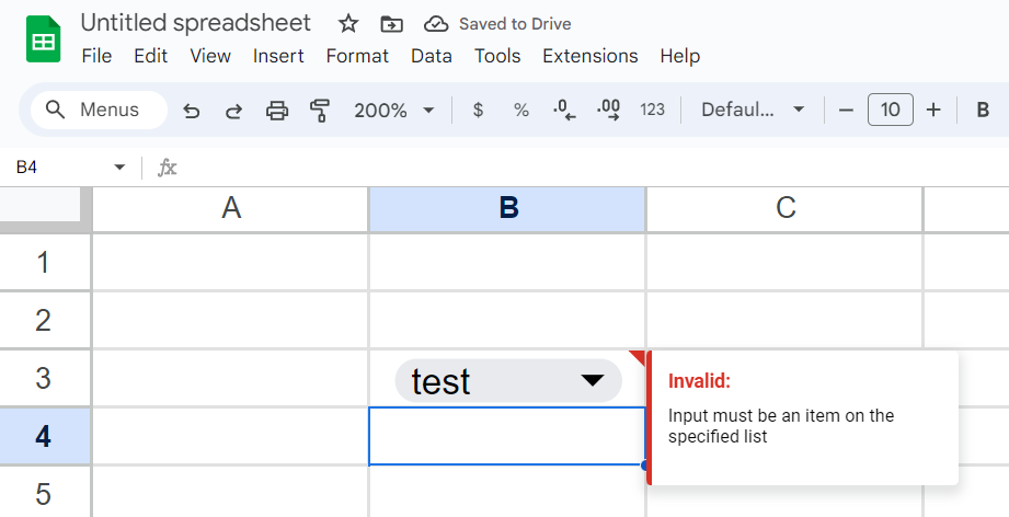
The result of an incorrect entry is as follows:
In the Digital Guide, you can find out how to edit Google Sheets drop-downs as well as more information on formatting cells in the article ‘Google Sheets: Conditional formatting explained simply’.
- Up to 50 GB Exchange email account
- Outlook Web App and collaboration tools
- Expert support & setup service

